Finite choices
A somewhat unconvenient answer to why you can't have it all
Summary: Unfortunately, there is no one singular “best tool for the job” when it comes to numerical simulation. Depending on the (mathematical) nature of your problem, certain methods give considerably better results than others. Interestingly, you can resort back to the theorem of “no free lunch” to explain why you can’t have an algorithm that does it all.
Introduction
No matter where you’re asking around within the industry nowadays, there’s a good chance that the majority of people will tell you that digitalization and hence simulation is an “evergreen” trend in product development.
In a world where there’s a company trying to sell you “the best simulation tool on the planet” around every other corner, you’d also be forgiven to think that some numerical methods are just clearly better than others.
Truthfully, every tool or method or behind it has its niche where it shines. The job as a scientist / engineer is primarily to find the best tool for the job whilst keeping an open mind. Otherwise you’d soon be too narrowed down on one solution, or in the words of the famous Abraham Maslow
“I suppose it is tempting, if the only tool you have is a hammer, to treat everything as if it were a nail.”
Finite Difference Method
This technique can be regarded as the most “primitive” alternative to solving this type of problems and dates back to its origins more than 100 years ago by Richardson
Now you’d be right to ask whether that wasn’t a little simple for notoriously hard to solve problems (by hand) and you’d be absolutely right.
In fact, the error of this approximation is of linear order with the step size, which is far from the best when talking about accuracy
On the other hand, the FDM gives a very universal way of tackling PDEs. You’d call it a jack of all trades, but master of none.
Finite Volume Method
In contrast to the FDM, we’re now not considering singular points or vertices of your domain, but rather a cell where inside a portion of the overall physics happens. This way of thinking is fundamentally different and one could argue that it stems from a more “engineering” way of thinking. The motivation stems from the idea that you would split an integral solution of a problem into a specific (finite) amount of subdomains, each with their own solution. This method is especially prominent in fluid dynamics, where dealing with conservation equations is quite common
Consequently, we are not considering differential forms of the physics considered as in the FDM, but rather the conservative form that describes the physics on the entire domain. One typical equation with a conserved quantity $\phi$ would then look something like:
\[\iiint\limits_V\frac{\partial \rho \phi}{\partial t} dV + \underbrace{\iiint\limits_V \frac{\partial}{\partial x_i} (\rho u_i \phi) dV}_{\text{Convection}} - \underbrace{\iiint\limits_V \frac{\partial}{\partial x_i} (\rho \Gamma_\phi \frac{\partial \phi}{\partial x_i} ) dV}_\text{Diffusion} - \underbrace{\iiint\limits_V S_\phi(\phi) dV}_\text{Source} = 0\]Again, we need to find some means of discretizing this expression in space (and time). Characteristic of the Finite volume Method is the application of Gauss’ divergence theorem so that the volume integrals become hull integrals over the faces of the domain:
\[\iiint\limits_V \frac{\partial u_i}{\partial x_i} dV = \oint\limits_{\partial V} u_i \cdot n_i dS = \oint\limits_{\partial V} u_i dS_i\]We now split the global domain into separate, finite subcells so that we can write the conservation equation using finite sums:
\[\oint\limits_{\partial V} (\rho u_i \phi)dS_i = \sum\limits_f \oint\limits_f (\rho u_i \phi)_f dS_i \approx \sum\limits_f \sum\limits_i \underbrace{\overline{(\rho u_i \phi)}_f}_\text{mid point rule} S_{if} = \sum\limits_f \sum\limits_i (\rho u_i \phi)_f S_{if}\]To this day, FVM remains a popular choice for dealing with flow phenomena of many sorts. But this method also is not without its flaws. We will try to sketch the most problematic in short. For now, reimagine the idea of FVM in terms of neighboring cells. You can then convince yourself that in a 3D domain, each volume shares a common face with a neighboring cell. Due to the way FVM is set up using Gauss’ theorem, the values of one cell needs to be reconstructed by the values on the faces. This leads to the problem that for one face, you have multiple values that the one on the face could assume. So how choose? This kind of discontinuity poses an important problem and there are many ways to deal with this. One way for example is to simply take the value of the upwind cell, which consequently is known as upwind differencing. This method, however being stable, can produce highly diffusive solutions which in turn is undesirable. There are other methods that tend to exhibit opposite behavior. Achieving both relative stability and low diffusivity is often more art than science.
One example for the tradeoff you have to make regarding stability and diffusivity is given in the figure below
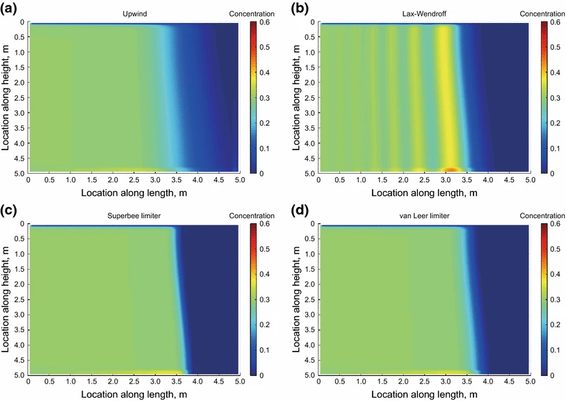
You can clearly observe that the schemes that preserve the sharp concentration gradient at about 3.5 m length tend to produce (unphysical) oscillations. In contrast, the typically diffusive upwind scheme keeps the overall concentration within the set bounds but produces a somewhat “mushy” zone around the shock area. This is a very typical setting and illustrates the difficulty of choosing an appropriate scheme for your problem.
Finite Element Method
The Finite Element Method has a history that is somewhat hard to sketch in a historically correct manner. Initially, the way of coming up with this method was also closely linked to a given problem similar to FVM, just in this case it was solid mechanics. You would similarly divide the domain into elements and calculate individual solutions each. The original formulation of the FEM was also very specific to static problems in mechanics, where you would assemble a stiffness matrix and solve it by common linear algebra.
However, state-of-the-art FEM does not share much of its DNA with what was just presented. It is rather a more powerful approach of dealing with all kinds of phenomena. The modern interpretation of this technique is known as the Galerkin Finite Element Method. This can in turn be further divided into continuous (CG-FEM) or discontinuous (DG-FEM) methods.
The basic idea more or less goes as follows: We are not trying to obtain the accurate solution of the problem in terms of the function itself, but are rather seeking a functional approximation - much of what you would do with a Taylor series (polynomial approximation) to an arbitrary function. The output of such a simulation is therefore not the actual function itself discretized in space, but rather the coefficients of the set of functions that you’re trying to approximate the solution with. As you might already have guessed, this is a much more mathematical way of thinking in contrast to the more hands-on approach how the method was originally conceived
The mathematics behind the FEM as well routes from another discipline, namely functional analysis. We here consider a so called variational formulation of a weak form derived from the problem at hand.
\[\int\limits_{\partial \Omega} \frac{\partial q}{\partial t} \phi_j dx + \int\limits_{\partial \Omega} \frac{\partial f(q)}{\partial x} \phi_j dx =0\]The weak form is obtained by integrating the PDE over the domain $\Omega$ and multiplying it with a so called set of test functions $\phi_i$. Here, the nonlinear terms that we encountered in the Finite Volume section are summarized in a differential operator $f(q)$. We then seek to approximate the exact function $q(x)$ that solves the problem by an approximate representation $\tilde{q}(x)$, comprised of certain basis functions $\Psi_i(x)$:
\[\tilde{q}(x) = \sum\limits_{i} a_i \Psi_i(x)\]Often enough, these functions are polynomials of special kind that possess certain properties regarding their definition range. One popular example are Lagrange polynomials that have the fundamental property of only taking the value 1 at one and 0 at every other node that comprise the geometry of one finite element.
Finally, as we are not modelling the problem exactly, we set the right-hand side equal to a residual that must tend to zero as we approach the real solution. Here, we achieve this by systematically approaching the right basis coefficients $a_i$.
As we can see above, there is also some integration that needs to take place here. That means we encounter the same problem that we had with the Finite Volume formulation - how do we calculate these numerically? Instead of converting these into hull integrals, we take a different approach here. We are here considering a finite set of elements that each contain a certain amount of nodes, depending on the element type. Within these elements, we use the Gauss quadrature rule to perform explicit integration. This can be formulated in a way that the integration yields even exact results for a certain choice of basis functions. So in some way, we again may thank one of the greatest mathematicians in history for letting us perform this difficult task, yet with a completely different approach.
Now what are the pitfalls of this approach? Depending on the choice of the function basis, the element size and the type of problem, we may encounter convergence issues much similar to the other methods. In this case, as we’re trying to minimize a certain residual, this value might not converge to zero, hence yielding a suboptimal approximation
Putting it all together
Leaving all good marketing aside - isn’t there one clear “winner” amongst those? Can’t there just conveniently be one method that does it all?
The answer to this question is at the same time remarkably simple and complicated at the same time. Wolpert and Macready have put this in a beautifully elegant way that has become famous as one formulation of a “no free lunch theorem”
“[…] for any algorithm, any elevated performance over one class of problems is offset by performance over another class. “
This fact about optimization algorithms (and this is what numerical PDE solvers ultimately are) gives a useful introduction and baseline to our following discussion. From this point, to simplify things, we will talk about techniques for numerical modelling of partial differential equations (PDEs) when mentioning the term simulation.
So when you’re trying to solve a physical phenomenon that is modelled by a PDE, you are not to expect that the (mathematically) optimal choice of algorithm for this problem will perform equally well in another type of problem. That is, in short, the simple part of our answer.
The more specific answer lies in the nature of PDEs. When talking about equations of second order - which, surprisingly, an overwhelming fraction of real world physical phenomena is covered by - we can make a classification into three separate types: hyperbolic, parabolic and elliptic. If you’re more into the mathematics behind, I suggest some sort of introductory book on analysis.
Depending on the terms occuring in the physics you’re modelling, it can be advantageous to chose one method over the other as some parts of the equation might impact convergence in a severe manner. For example, the Continuous Galerkin Finite Element method has been used successfully for dealing with elliptic and parabolic problems, especially for solid mechanics and heat conduction problems. However, this very method struggles when modelling hyperbolic problems such as the Navier Stokes equations, or in general physics involving convection for that m atter
So interestingly enough, our no free lunch theorem (in a much more hand-waving and non rigorous way) does hold again for making up one’s mind for choosing the right tool for the job. You can either try to do the calculations by hand - which often enough gives surprisingly valid results with only a few simplifications - or you can resort back to the numerical methods we’ve lined out. Though, you most likely not get around thoroughly investigating the nature of your problem if you want to obtain accurate results in reasonable time. So again, there’s no free lunch with either choice.